
Chapter 4 Working with R
This section will be kept brief as there is a large set of introduction material online. For example this online book: “Introduction to R”8. There are indeed a few principles in “Classic R” that should be understood such as creating R objects (section 4) and using basic R functions.
In this chapter:
- Creating used-defined
Robjects - Functions and their arguments
- Vectorization
- Data frames tabular format
- Generating data
- Simple graphics with
plot()
4.1 Creating R objects
User-created R objects are a method to handle data. It can be thought of as two actions:
- Read the data into a container, or jar
- label the jar with the content
Regardless of the size of the data (and perhaps with a little magic?) the container will adopt the required size to contain all of the data.
The user will then define a name for the container to easily call it back later.
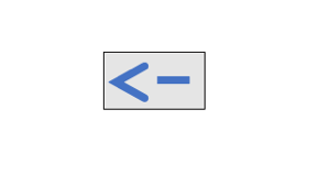
Figure 4.1: The assignment operator <- is used to create R objects.
NOTE
The assignment operator can be replaced with the equal sign = in most cases but “R purists” prefer the standard <- assignment code.
For a more complex discussion see What are the differences between “=” and “<-” assignment operators in R?9
Here is a simple illustration: we’ll place the word strawberry into an jar called jam. In order to do the job we need to use the “assignment” symbol <- that could be read as “assign…” or “place into” or “read in” etc. Since strawberry is a word and not a number it has to be placed between quotes.
we now have an R object called jam that contains the character string strawberry. In the top right panel in RStudio the new object is now listed as shown in figure 4.3.

Figure 4.2: A jar as a metaphor for an R objects.
As we just saw, characters have to be placed within quotes.
The following data types occur often with routine R calculations:
- Numeric
- Integer
- Complex
- Logical
- Character
An R object can contain many types of data. It is easier to understand this with numbers. Let’s make another object: we’ll assign the number 12 to an object labeled dozen. Since 12 is a number we do not use quotes.
Since dozen contains and represents the number 12 we can also use mathematical operators on it. for example we can calculate how much are 2 dozens: the result is calculated by R using dozen as a variable.
[1] 24The result will be printed on the screen. Since there is only one value, the first line on the result is [1].
The choice of the label (or name) of the R object should be helpful. Here dozen is very specific and one would not want to use that label for containing any other number than 12. For example, a baker’s dozen, which is typically 13 should be given a suitable variable name such as bakerDozen or baker_dozen.
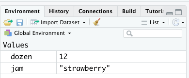
Figure 4.3: R objects are conveniently listed within the Environment Tab in RStudio.
Obviously since dozen represents a number, it can be used to multiply or divide.
Let’s choose a more generic label. Some people like to add my as part of the chosen name to make sure that they are not inadvertently using the same name as another program. for example let’s use myNum to represent my number:
We can again make use of this object that will replace the value it contains. Here are some examples with arithmetic operators: add, subtract, multiply, divide. (See Appendix @ref=(arithmeticoperators).)
[1] 24[1] 0[1] 144[1] 1We can also ask if the two objects are “equal”, a question that can only result as TRUE or FALSE. This comparison requires using relational operators (see Appendix B.3.) It is noteworthy that such comparison is not limited to objects containing numbers. It is important to notice that the symbol is made of 2 “touching” equal signs: == not to be confused with the equal sign itself =.
[1] TRUE
Figure 4.4: A dozen often referred to eggs.
Exercise: calculate a price
The price of one egg is 20 cents.
The price of a dozen is discounted 10%.
We want to buy 3 dozen.
How much will this cost?
Can you write the code to easily change the number of dozen purchased? or if the discount is changed later?
# here are some hints

egg <- 0.2 # 20 cents in $
dozen <- 12
discount <- 0.10 # 10% in decimal
myNum <- 3 # how many I want now
Of course this could be calculated with just the numbers. But it makes computing changes easier if we use variables. Later we can change the variable assignment.
Price without discount: $ 7.2
Discount: $ 0.72
Discounted price = $ 6.48
CAUTION
R objects cannot have a name that start with a number and cannot contain a dash as it is interpreted as a minus sign.
The name of an object must start with a letter (A–Z or a–z) but can include letters, digits (0–9), dots (.), and underscores ( _ ). R is case sensitive and discriminates between uppercase and lowercase letters in the names of the objects, so that a and A can name two distinct objects (even under Windows).
4.2 Functions and their arguments
We just saw examples on how to use R with numbers to do some calculations. More complicated calculations, and computations, are handled with functions many of which are installed as part of base R installation. More functions can be added as we’ll see later when we add R packages.
Functions perform a task to “accomplish something.” The “something” could be the transformation of data, for example calculating the logarithmic value of a provided number. Most of the time the function returns and output.
Therefore one can think of a function taking an input and usually providing an output.
Figure 4.5: A function typically takes input and provides output.
The input is provided in the form of argument which can be R objects, variables, numbers, etc. A function will typically have a default behavior that can be modified with optional arguments.
A function is always written as its name followed by parenthesis, even if these remain empty. For example the function to list all the R object currently within the workspace is the list function and it written as ls().
Figure 4.6: A function is always written with parenthesis even if they remain empty.
Most functions will have a default behavior as determined by default arguments. For example, the function dir() without any argument by default will show the content of the current directory.
Additional arguments and options may be added to a function to modify its behavior. The input is typically one of the arguments provided. Arguments can be anything expected by the function and can be numbers, filenames, but also other objects. The meaning of each required or optional argument may differ depending on the function and can be looked up in the documentation.
Figure 4.7: A function has default arguments. Options and additional arguments may modify its behavior.
4.3 Built-in functions
An R function is invoked by its name, then followed by parenthesis. Parenthesis contain mandatory or optional arguments to pass to the function. Parenthesis are always written even if they remain empty.
4.3.1 list: ls()
For example we can now list the R objects that we created above with the function ls():
[1] "colorize" "discount" "dozen" "egg" "jam" "myNum" 4.3.2 class()
We can verify the type, or class of these variables with the function class()
[1] "character"[1] "numeric"4.3.3 combine: c()
The combine function is essential in R.
For example the following three numeric values are combined into a vector. (More on vectors below, section 4.6.1.)
[1] 1 2 3Since we did not assign to a user-defined object or a variable name the output is immediately printed out on the R console and will not be remembered.
Here is the same vector assigned to variable v
This time no out put is produced but the data is stored in memory and can be called back.
However, it is possible to obtain both actions at the same time: placing the assignment code within parenthesis:
[1] 1 2 34.3.5 Working directory: getwd() and setwd()
In section 3.4 we saw how to choose a new directory or return to it.
Functiongetwd() will get the working directory and print it on the console.
Function setwd() will take as argument the absolute or relative path
to the new chosen directory as defined by your operating system. Mac, Unix and Linux users use the forward slash (/) as a separator. This also works in Windows. However Windows users need to double back slashes (\\) if they use the backslash (\) as a separator. See Appendix C for sample code example that is also suited for Windows users.
4.4 Getting help
R provides extensive documentation. Depending on the installation method or how you access R the results may appear either in plain text within the R console, an HTML page, or within the Help tab on RStudio, etc.
For example, entering ?c or help(c) at the prompt provides documentation of the combine function c().
NOTE
Within help, ... often means that arguments can be passed along by other functions. index{Symbols!…}
4.5 Vectorisation
R calculations are “vectorized” in the sense that any calculation can be applied to all elements of e.g. a vector. For example:
[1] 10 20 30[1] 0.5 1.0 1.5This is a very important aspect of R.
4.6 More complex data
There exist other types of more complex data that R can handle, most of them can be tabular or multidimensional:
- Vector
- Matrix
- List
- Data Frame
Tabular data is a very common form to collect information and most useful in data analysis.
4.6.1 Vectors
We already created a one-dimensional vector v above containing numeric values. But vectors can also contain characters or logical data. However, all data in one vector have to be of the same nature.
For example here is a vector made of characters:
4.6.2 Matrix
A matrix is a collection of data elements arranged in a two-dimensional rectangular layout. All elements have to be of the same nature, e.g. numeric or character.
The function matrix() can be used to create a new matrix object.
     [,1] [,2] [,3]
[1,]    1    3    5
[2,]    2    4    6
However, some more information needs to be given, for example how many rows should the matrix have, this is done by the nrow= option. Obviously the number of elements given should be in the number of expected row by columns. The default values are nrow = 1, ncol = 1 and the default filling method is by column since the default is byrow = FALSE.
EXERCISE
Try to change some of the defaults. For example change byrow = FALSE to byrow = TRUE.
Your results:
---------------------------------------------------

---------------------------------------------------

---------------------------------------------------
4.6.3 Combining vectors to create a matrix
Another way to create a matrix is by combining vectors of the same length with the functions cbind() or rbind() to combine by column or row.
EXERCISE
Try these commands on the vectors v and vc - for example:
Your results:
---------------------------------------------------

---------------------------------------------------

---------------------------------------------------
What happened when using both v and vc
(hint: class().)
---------------------------------------------------

---------------------------------------------------

---------------------------------------------------
4.7 Dataframes
Dataframes are a type of table that allows each column to contain a different variable type. For example one column can contain characters and another column can contain numbers.
This type of tabular data is extremely useful in data analysis.
We can use the function data.frame() to construct a dataframe starting with and combining vectors.
# num: a vector if numbers
num <- c(2, 3, 5)

# let: a vector or letters
let <- c("aa", "bb", "cc")

# tf: a vector or logicals true or false
tf <- c(TRUE, FALSE, TRUE)

 # df is a data frame
df = data.frame(num, let, tf)
We can inquire about df: the class of the object, its dimensions, the name of the headers for the columns.
[1] "data.frame"[1] 3 3[1] "num" "let" "tf" 4.7.1 Dataframe manipulation
As just as simple demonstration we’ll change the name of the rows.
For now the dataframe looks like this:
  num let    tf
1   2  aa  TRUE
2   3  bb FALSE
3   5  cc  TRUE
and if we ask the name of each row we get the current list:
[1] "1" "2" "3"In R things can change by reassigning new values, so we can indeed change the row names with the function**rownames() and giving new values. For example:
     num let    tf
row1   2  aa  TRUE
row2   3  bb FALSE
row3   5  cc  TRUE
In the same way we could change the column names:
Note: functions
row.namesandrownamesexist for rows, but onlycolnamesexist for columns.
In this final version the data itself is not altered but we changed both the column and row names:
     numbers letters logical
row1       2      aa    TRUE
row2       3      bb   FALSE
row3       5      cc    TRUE
4.8 Generating data
There are many ways to generate data from within R as series of numbers, in sequence or as random numbers. This section is purposefully kept simple.
4.8.1 Regular sequences
The generation of numbers in sequence can be useful to create lists.
The following command will generate an object with 10 elements; a regular sequence of integers ranging from 1 to 10, saved wihtin variable x thanks to the operator :
[1] 1 2 3 4 5 6 7 8 9 10Various options can be used to alter the results, for example requesting 11 values, starting with 3 and ending at 5.
[1] 3.0 3.2 3.4 3.6 3.8 4.0 4.2 4.4 4.6 4.8 5.04.8.2 Repeat and sequence functions:
It may be useful to print a number multiple time. This can be done with the rep() function. For example:
[1] 1 1 1 1 1 1 1 1 1 1 1 1 1 1 1The function sequence() creates a series of sequences of integers each
ending by the numbers given as arguments.
[1] 1 2 1 2 3 1 2 3 4 1 2 3 4 5For clarity here is the result with * separators added:
[1] 1 2 *1 2 3* 1 2 3 4 *1 2 3 4 5*To understand this output it is useful to also remember that 2:5 means 2, 3, 4, 5 and that the function will apply to each of these digits in turn.
4.8.3 Levels: gl() and expand.grid()
These two functions are very useful for creating tables containing experimental data.
The function gl() generates “levels”series of “factors” or “categories” as values or labels. The following example will generate 4 each of 2 levels:
[1] Control Control Control Control Treat   Treat   Treat   Treat
Levels: Control Treat
The function expand.grid() creates a data frame with all possible
combinations of vectors or factors given as arguments.
This example
   h   w    sex
1 60 100   Male
2 80 100   Male
3 60 300   Male
4 80 300   Male
5 60 100 Female
6 80 100 Female
7 60 300 Female
8 80 300 FemaleNote: The arguments are rotated as a function of their position in the command.
How many lines is the table (not counting the header? (hint: row numbers)
----------------------------------The use of seq() can also be useful in this context.
EXERCISE
Try the following examples.
How many lines is the table (not counting the header? (hint: row numbers)
----------------------------------Add one more variable treatment = c("control", "drug")) and see how much the table expands:
How many lines is the table (not counting the header? (hint: row numbers)
----------------------------------Note: the function dim() can be applied directly as well, for example:
4.8.4 Random numbers
Most of the statistical functions are available within R such as Gaussian (Normal), Poisson, Student t-test etc.
To generate random numbers, the function based on the Normal distribution we use the function rnorm() (r for random and norm for Normal.) The number of desired random numbers is given as argument.
Since these are random, the answers are never the same!
EXERCISE
Perform the following command requesting a single random number a few times (e.g. 5 times) in a row:
Do you get the same result every time?
[ ] Yes [ ] No
To provide means of reproducible the function set.seed() can be used to obtain the same result every time. The seed is a number chosen by the author. Here is an example selecting three numbers.
[1] -0.13592452 -0.04079697 1.01053901[1] -0.13592452 -0.04079697 1.01053901[1] -0.13592452 -0.04079697 1.01053901However, changing the seed value will change the results:
[1] -0.5121391 2.4851837 1.0078262Important note10 “[these] Pseudo Random Number Generators because they are in fact fully algorithmic: given the same seed, you get the same sequence. And that is a feature and not a bug.”
One R method for choosing letters at random is with the function sample(). The term LETTERS represents the alphabet and is built-in R.
[1] "Q" "E" "K" "C" "P"[1] "T" "P" "H" "Z" "A"In the same way as before setting a seed will reproduce the same result every time.
[1] "Q" "E" "A" "J" "D"[1] "Q" "E" "A" "J" "D"4.9 Conditional statements
Making choices or decisions are what conditional statements are all about in programming.
There are multiple ways of writing a conditional statement in R using different functions
4.9.1 Function ifelse()
Function ifelse() has the same functionality as the IF statement in Excel and required 3 arguments:
- a logical test that is either
TRUEorFALSE - an answer if the logical test is
TRUE - and alternate answer if the logical test is
FALSE
This is best understood by an example:
# Logical test is TRUE: print first option
ifelse(5 > 4, "YES! 5 is greater than 4", "NO! 5 is not smaller than 4")
[1] "YES! 5 is greater than 4"# Logical test is FALSE: print second option
ifelse(5 <= 4, "YES! 5 is greater than 4", "NO! 5 is not smaller than 4")[1] "NO! 5 is not smaller than 4"This will be revisited later in the Tidyverse section (10.4.1.)
Other conditional statements can be learned elsewhere. For example:
- MODULE 4.5 Conditional Statements in R (Utah Sate Univ.)11
- Conditional statements and loops in R12.
4.10 Simple graphics with plot()
We will create a very simple graphic output from generated random numbers:
Create a data vector of 100 random numbers (note: if you choose the same seed number your final plot will be identical.)
The plot() function will create a simple scatter plot with circles as the default symbol.
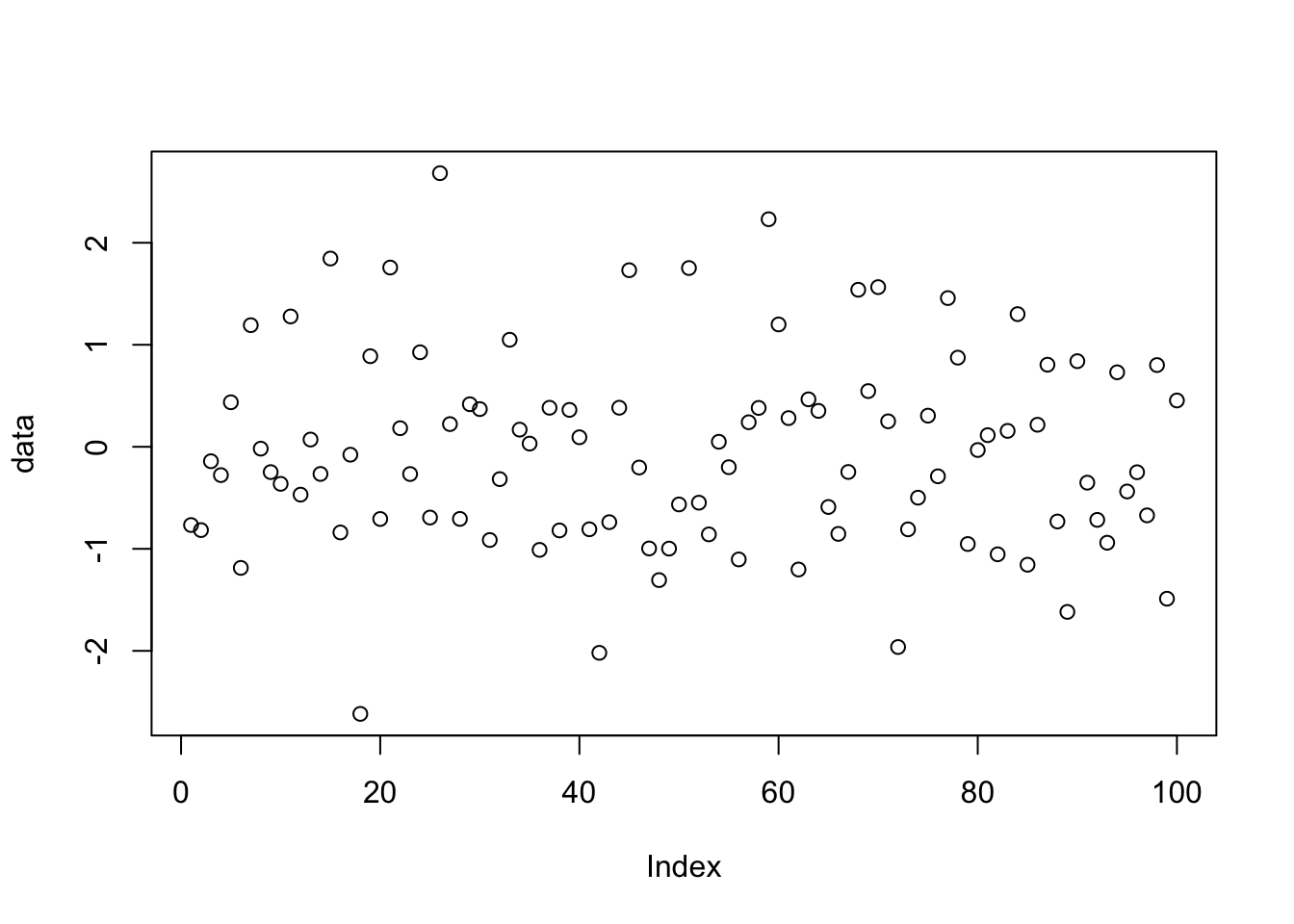
Figure 4.8: Function plot() automatically generated scatter plot.
It is possible to include more than one plot on the same figure/page with the parameter function modifying the number of rows and columns planned for plotting: par(mfrow=c(1,1)) by default.
As a brief example we’ll replot these data points as points, lines, both, and overlay. The labels for the axes are rendered blank to make the final layout less cluttered.
par(mfrow = c(2,2))

plot(data, type = "p", main = "points", ylab = "", xlab = "")
plot(data, type = "l", main = "lines", ylab = "", xlab = "")
plot(data, type = "b", main = "both", ylab = "", xlab = "")
plot(data, type = "o", main = "both overplot", ylab = "", xlab = "")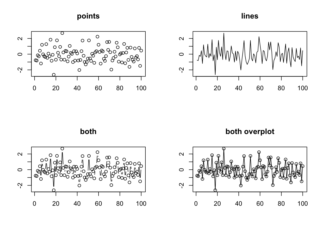
Figure 4.9: Split screen plots.
Afterwards it is useful to reset the number of plots per page to 1:
Other types of default plots are available. For example a box plot.
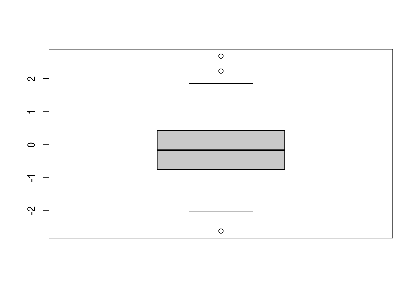
Figure 4.10: Function plot() automatically generated boxplot.
R default graphics are useful for exploring the data. However, more modern additional packages can be added to make plots more appealing while at the same time trying to make it easier to create them.