Chapter 13 Markdown and Reproducible research

Reproducible research is becoming a vast field. This chapter is to provide a flavor of what’s possible in creating a “live” document for data analysis. There are many sources online, here is one from a 6-hour workshop from the “Monash Bioinformatics Platform”: Reproducible Research in R ³⁹ (2019-07-25).

What is Reproducible Research?⁴⁰

Research is considered to be reproducible when the exact results can be reproduced if given access to the original data, software, or code. Reproducible research is sometimes known as reproducibility, reproducible statistical analysis, reproducible data analysis, reproducible reporting, and literate programming.

Literate programming is simply telling a “story” with the embedded code which is “rendered” in the final output.

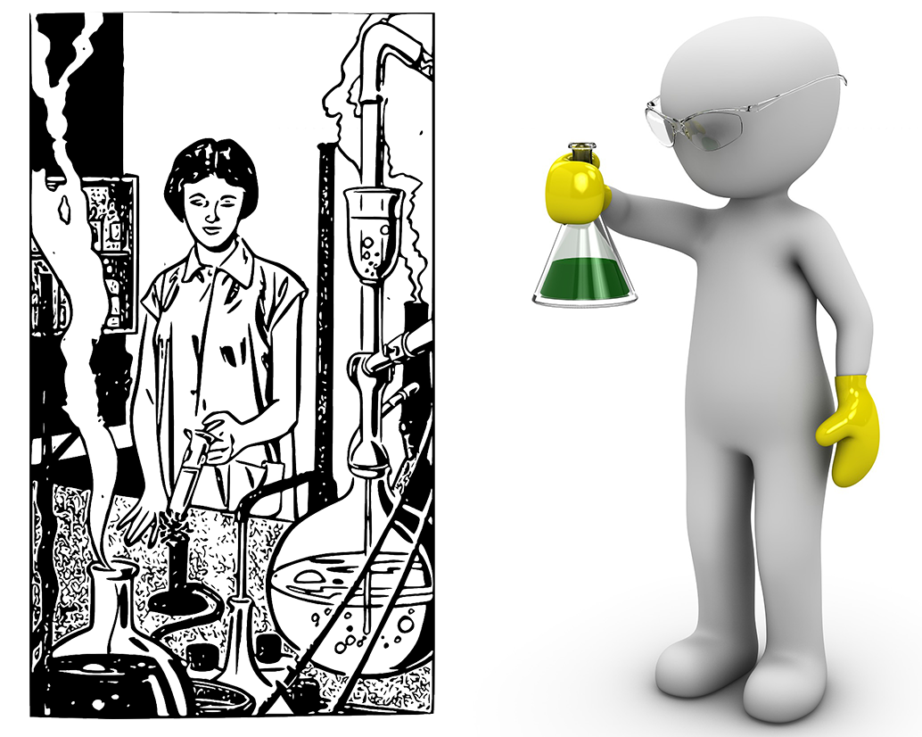
Figure 13.1: Reproducible research is more about computer analysis, replicable research is about reproducing research results.

Reproducible research usually refers more to the analysis of the data, while research that is replicable is the idea that research results can be reproduced by independent researchers using different methods.

A course on reproducible research using `R`
Name	Course Web site
`R` for Reproducible Research	https://annakrystalli.me/rrresearch/index.html

13.1 Markdown

What is markdown? Markdown is a lightweight markup language with plain-text-formatting syntax, created in 2004 by John Gruber with Aaron Swartz.⁴¹ (Note the play on words between markdown and markup!)

The philosophy or markdown is described by John Gruber on his web site: “DARING FIREBALL”⁴².

At its origin, John Gruber created markdown to easily create HTML pages with an easy syntax. The markdown document is a plain text file that in the end is used as a source to create an HTML page.

This very document is being written with the help of markdown!

A web page is written un HTML or “Hyper Text Markup Language” and its syntax requires a lot of characters to specify a format. The name “markdown” is a play on word and its syntax is very easy. Here is an example to make a word bold:

HTML: <b>word</b>
Markdown: **word**

Another more remarkable example would be the “heading” as it is used on the web but also in MSWord as a section title:

HTML: <h1>heading1</h1> -> requires 9 characters on both sides of heading1
Markdown: # heading1 -> requires a single character!

The result is that text files that are formatted in markdown can be read “as is” very easily, while a page of HTML code would be much harder for a human to read “as is”. In fact that was a key design goal: readability.

13.1.1 Markdown syntax

The basic syntax is illustrated on this page: www.markdownguide.org/basic-syntax/⁴³

The basic markdown syntax can be summarized in a short table from https://www.markdownguide.org/cheat-sheet/⁴⁴.

Basic Markdown Syntax
Element	Markdown Syntax
Heading	# H1 ## H2 ### H3
Bold	bold text
Italic	italicized text
Blockquote	> blockquote
Ordered List	1. First item 2. Second item 3. Third item
Unordered List	- First item - Second item - Third item
Code	`code`
Horizontal Rule	`- - -`
Link	`[title](https://www.example.com)`
Image	`![alt text](image.jpg)`

Extended syntax can be useful for making tables (such as the table describing basic markdown) or footnotes and listed further down on the same guide page.

Basic and most extended markdown syntax are included in RStudio.

Interactive tutorial

One easy way to learn how to use markdown is to go through the very easy interactive exercises dynamically rendered in the free interactive tutorial at www.markdowntutorial.com/ available in English, Spanish, French, Korean, and Japanese.

In turn RStudio created a method to add code within a markdown file which is then called an “R markdown” file.

Regular markdown can easily be learned from the above links, the next section will provide details on R markdown.

13.2 R markdown magic

Before experiencing the Magic of R markdown it is necessary to have an even rudimentary understanding of “plain” markdown - see previous section 13.1.1.

Markdown allows a document to be formatted easily but Rmarkdown provides the means to create a dynamic document that makes it easy to maintain both the narrative (text, story, information) and the analysis in the form of computer code that is woven within the file and can automatically embed data, tables and even plots and graphs automatically. Since this is all automated, if the original data is changed, converting the Rmarkdown document once more to a final output format (HTML,PDF, MSWord) will recompute and update everything, literally with one click!

This is a valuable tool in the context of Reproducible research as a paper could be completely self-contained within an Rmarkdown document: the story, the analysis code, and the figures (automatically generated by the analysis code.)

The free online book R Markdown: The Definitive Guide ⁴⁵ by Yihui Xie, J. J. Allaire, Garrett Grolemund (2020-04-26) should prove a very valuable reference.

See more resources in Appendix H.

13.2.1 Before your start

Some packages are needed to create output from R markdown documents which you can install in advance, for example with:

install.packages(c("knitr", "rmarkdown", "markdown"))

However, the newest versions of RStudio will prompt you if you want to install a package that is necessary but not yet installed.

The knitr package is used to transform the R markdown .Rmd file into a beautifully rendered document in various formats. The knitr package name reflects the “knitting together” (weaving together) the text and the embedded literal programming code and at the same time makes things look a lot more “neater.”

13.2.2 How to create an R markdown file

TASK: open an R markdown template

To follow these exercises create a new R markdown file with the menu cascade:

File -> New File -> R Markdown...

In the new window replace "Untitled" with a title for your document.
Keep HTML selected as the “Default output format”
Press OK
Save the file now (or later) and provide a name for the file.
The new file will have a filename extension of .Rmd

The top of the file will look something like this:

---
title: "Test1"
author: "My Name"
date: "7/22/2020"
output: html_document
---

WARNING! DO NOT TOUCH THIS SECTION YET!

This section is a special header that provides instructions on how to export the final document (output: html_document) and can be changed with further instructions. This is formatted in a simple language called YAML⁴⁶.

The rest of the page is meant to write text with or without (regular) markdown formatting, but also can contain R code that can be shown or hidden, executed or inert. It is worth pointing out that RStudio supports many more languages that just R and are called “engines” in that context⁴⁷.

13.2.3 Adding R code

The whole purpose of an .Rmd file is to tell a story with markdown and perform the analysis at the same time when it is rendered. This is accomplished by adding R code “chunks” within the file that will be evaluated when the weaving/knitting of the file output is done.

To add R code we can use the “Insert” button on Rstudio bar, or simply write the code between special characters that specify that it is code and not just text in this way:

```{r}
# Here goes the R code
V <- c(1:10)
```

A name can be given to the “chunk” and a various number of options that can modify the results of what happens when the final document is knitted. For example the code could be running but not shown in the final document by adding echo = FALSE. (Complete chunk options list(PDF)⁴⁸.) It is easier to see an example:

---
title: "Tiny Rmd"
output: html_document
---
In R it is possible to tell a story and weave computer code 
to perform an analysis at the same time by adding "chunks" of code. 
This code will create a vector and take the log10 of each value

```{r mychunk, eval=TRUE}
  # This chunk will be computed
  V <- c(1:10)
  log10(V)
```

The values are automatically printed

When the knit button is pressed the rendering in HTML will look like this:

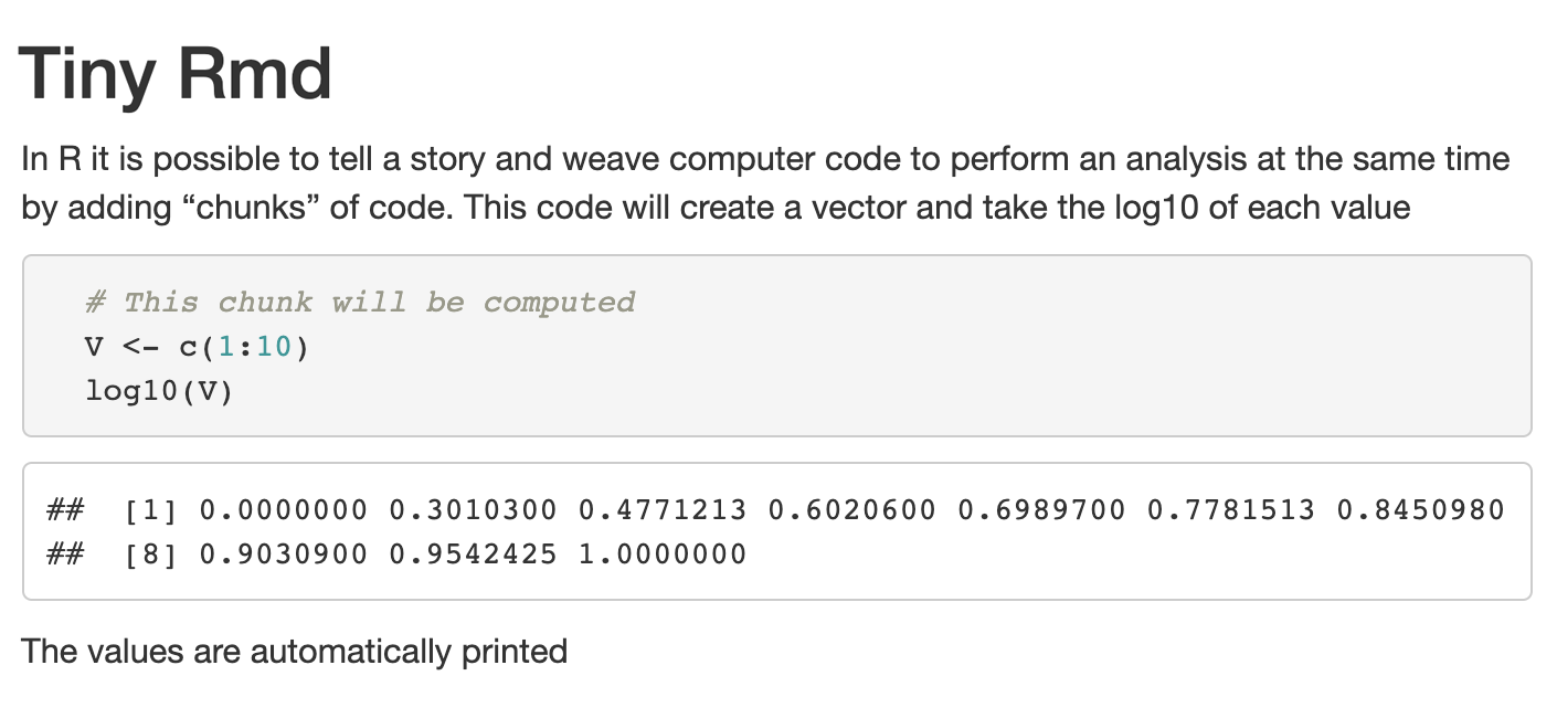
Figure 13.2: HTML output of Tiny Rmd as knit output.

Exercise 13.1 Exercise

You can try to Copy/Paste the text for Tiny Rmd file above and paste it within a new .Rmd file (details in section 13.2.2,) replacing all of the demo content with the pasted text of Tiny Rmd. Then press the knit button and see the result!

13.2.4 Very tiny Rmd file: Inline code

Here is one of the most useful and somewhat advanced ways of using R code to avoid “Copy/Paste” of information that may be unstable and could change over time. For example the size (length, dimensions, etc.) of the provided data for R to analyze may be updated with new information.

Here is an example of a very small file that shows how R code can be embedded within the text and rendered in the context of reporting.

The YAML is very minimal
the first line prints out 5 letters from the English alphabet (LETTERS is predefined in R.)
The second line embeds two commands separated by a semi-colon ; that first defines a vector of numbers, and then computes the sum of the numbers.
In both cases the results are shown in bold.

---
title: "Tinyest Rmd"
output: html_document
---
Some random letters: **`r sample(LETTERS, 5)`**  

Let's make a vector and add all its numbers: 
**`r vec <- c(1:10); sum(vec)`**.
Only the results will show on the final print.

Pressing the RStudio Knit button will convert this .Rmd file into an HTML document.

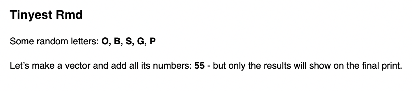
Figure 13.3: HTML output for Tinyest R markdown conversion with Knit button.

Exercise 13.2 Exercise: The story of vector V

You can read the “magical story of vector V” from the the text in Appendix I that you can Copy/Paste into a new .Rmd file.

This is a way to learn by example about R code chunks and the very useful inline R code.

The magic is perhaps in the story, but more importantly it is also the demonstration of weaving text and code together in a single rendered document.

13.3 Other formats

The two formats that should work by default are HTML and Word. Most people would be interested in created a PDF but that requires the installation of a typesetting engine called “LaTeX” (pronounced “lay tek.”) In the early days this required the installation of software independent of RStudio that was heavy in size in the multiple Gigabytes (most are 5Gb or more.)

TinyTex for PDF

Fortunately there is now a special package called TinyTex that is much easier to install and much smaller in size at about 150Mb only. Information on the package and installation instructions can be found on yihui.org/tinytex/ (Yihui Xie is a software engineer at RStudio and author of knitr and Tinytex among others.)

Optional Installation TinyTex

The tinytex R package (written as bold, lower case) is used to install TinyTeX, its distribution version of “Latex” (pronounce “la-tek.”)

The installation is simple and requires 2 easy steps:

install the tinytex package.
use tinytex to install the TinyTeX distribution.

Here are the 2 commands to accomplish this⁴⁹ plus a third, commented command to uninstall if necessary.

install.packages('tinytex')
tinytex::install_tinytex()
# to uninstall TinyTeX, run tinytex::uninstall_tinytex()

13.4 A word on YAML

YAML is a language and therefore can be overwhelming, confusing and offer too many “options” (as most computer languages do.)

However, as the language of the header of the .Rmd files there are just a few things that are of real importance.

13.4.1 Limits

The header is limited by three dashes at the top and at the bottom. Beyond this limit it become the realm of R markdown.

13.4.2 Indentation and White space

White space is part of YAML’s formatting. Unless otherwise indicated, newlines indicate the end of a field.

Indentations:
* used to structure a YAML document.
* only use white space, never Tabs.
* in .Rmd indentation is 0, 2 or 4 spaces exactly.

13.4.3 Automatic modifications

Parts of the YAML header may change automatically depending on actions. For example, suddenly decided to knit a simple document to a new format will modify the output statement.

---
title: "Tiny Rmd"
output: html_document
---

In the original version the keyword output: line contains a colon (:) followed the expected document format.

After requesting a different format, the output will automatically be changed, each time. The new output: line is now ending with a newline and the now multiple formats are each on a separate line indented by exactly 2 spaces (not 1, 3, or 4, or tab all of which would cause an error later.) The last document format requested will always be the one shown on top in the first indented line, updated each time the document is knitted.

---
title: "Tiny Rmd"
output:
  word_document: default
  html_document: default
  pdf_document: default
---

13.4.4 Quotes

Test should pruudently be placed within double quotes, for example title: "Tiny Rmd" even though title: Tiny Rmd would also work. Adding the quotes as it is done by default prevents text with special characters to cause an error.

13.4.5 Date

When a new .Rmd file is created it is given the date true on that moment and would not change later.

It is possible to use code so that the date is updated each time the document is knitted into a final format. Here are options to format the date at that moment:

date: "Last Updated:" `r Sys.Date()` "
date: ' `r Sys.Date()` '
date: " `r format(Sys.time(), '%d %B, %Y')` "
date: " `r format(Sys.time(), '%Y, %B %d')` "

Which would result in the following formats:

date: "Last Updated: 2022-07-07"
date: '2022-07-07'
date: "07 July, 2022"
date: "2022, July 07"

13.4.6 YAML resources

For further reference see the online book R Markdown: The Definitive Guide that details advanced options for YAML headers:

HTML content: https://bookdown.org/yihui/rmarkdown/html-document.html
PDF content: https://bookdown.org/yihui/rmarkdown/pdf-document.html
MSWord: https://bookdown.org/yihui/rmarkdown/word-document.html
General output formats: https://bookdown.org/yihui/rmarkdown/output-formats.html

An interesting way to see if your YAML header has any errors:

YAML validator: http://www.yamllint.com/

https://monashdatafluency.github.io/r-rep-res/↩︎
https://www.displayr.com/what-is-reproducible-research/↩︎
https://en.wikipedia.org/wiki/Markdown ↩︎
https://daringfireball.net/projects/markdown/↩︎
https://www.markdownguide.org/basic-syntax/↩︎
https://www.markdownguide.org/cheat-sheet/↩︎
https://bookdown.org/yihui/rmarkdown/↩︎
YAML is a recursive acronym that means “YAML Ain't Markup Language”↩︎
Command names(knitr::knit_engines$get()) will print supported languages (‘engines’). Install knitr package first.↩︎
https://rstudio.com/wp-content/uploads/2015/03/rmarkdown-reference.pdf ↩︎
https://yihui.org/tinytex/↩︎