Chapter 7 Creatinine adjustment

Many of the NHANES samples are derived from urine sample analysis. In order to compensate for most variations between individuals it is often necessary to proceed to an adjustment with the level of creatinine a metabolite that has a rate of excretion rather constant and can serve an an indicator of urine dilution.

In this chapter:

Creatinine adjustment rationale
Download and explore creatinine data
Converting weight/volume units
Merging and reducing data
Computing and saving creatinine adjustment

An older NHANES document had information about this process:

The concentrations of environmental chemicals per whole weight of serum are also on the laboratory file and can be used for comparison with other published studies that have investigated these chemicals.

The current NHANES urine collection protocol provides ‘spot’ urine samples because these are collected at different times of the day (depending on the examination session) and only one specimen is collected from each survey participant. The laboratory measures of environmental chemicals in urine are provided on the data files as concentrations per volume of urine. Each data set for environmental chemicals measured in urine, also includes a variable for urinary creatinine concentration.

Urine dilution may vary markedly from person to person, time to time, and because of other conditions, including fluid consumption, physical workload, and health. Creatinine is produced as a result of muscle metabolic processes, and excreted from the body at a fairly constant rate (though extreme diets may affect urine creatinine levels). The effect of urinary dilution can be accounted for by determining the amount of the environmental chemical per amount of urinary creatinine in a given volume of urine.

The equation for creatinine adjustment is:

Analyte concentration per gram of creatinine =

Concentration of environmental chemical in urine (wt/vol)
  ————————————————————————————————————————————————
   Concentration of creatinine in urine (wt/vol)

WARNING Creatinine is related to lean body mass and renal function of individuals, and varies by age, gender, and race/ethnicity group.

It is recommended that one compare the creatinine-corrected environmental chemical concentrations among individuals of similar demographic groups rather than the whole population because urinary creatinine levels differ according to age, gender, and race/ethnicity. Alternatively, multiple regression analyses can be conducted using urinary creatinine as an independent variable (in addition to variables for age, gender, and race/ethnicity), so that the environmental chemical concentrations comparisons can be based on adjustment for urinary dilution and demographic differences.

The current NHANES web site no longer has this information in this format. It is available as a copy in a page titled “Using Blood Lipid or Urine Creatinine Adjustments in the Analysis of Environmental Chemical Data”²² as the link within that page titled “Key Concepts about Blood Lipid or Using Urine Creatinine Adjustments of Environmental Chemical Data”²³

I have archived both pages at archive.org to preserve the availability of these pages. Searching with the original links within the archival site will retrieve these original files.

7.1 Creatinine data

The 2015-2016 document file is listed as ALB_CR_I.doc as it also contains information for albumin.

NHANES 2015-2016 albumin/creatinine data
Data File Name	Doc File	Data File	Date Published
Albumin & Creatinine - Urine	ALB_CR_I Doc	ALB_CR_I Data [XPT - 539.8 KB]	Updated June 2019

The data file contains 8608 data points (328 missing.)

The listed codes within ALB_CR_I.doc are:

Codes for albumin and creatinine ALB_CR_I file
Code	Description
SEQN	Respondent sequence number
URXUMA	Albumin, urine (ug/mL)
URDUMALC	Albumin, urine comment code
URXUMS	Albumin, urine (mg/L)
URXUCR	Creatinine, urine (mg/dL)
URDUCRLC	Creatinine, urine comment code
URXCRS	Creatinine, urine (umol/L)
URDACT	Albumin creatinine ratio (mg/g)

7.1.1 Downloading, merging PFAS and creatinine

As an example we’ll continue working on the PFAS_I urine metabolite and therefore we need to combine it with the creatinine data, again with the SEQN individual column. index{urine metabolite}

# Download NHANES ALB_CR_I 2015-2016 data to temporary file    
download.file("https://wwwn.cdc.gov/nchs/nhanes/2015-2016/ALB_CR_I.XPT", 
              tf <- tempfile(), 
              mode="wb")
# Create Data Frame ALB_CR_I From Temporary File
ALB_CR_I <- foreign::read.xport(tf)

Once the ALB_CR_I data frame is created we can merge it with the PFAS_I data frame.

# Merging PFAS and total cholesterol TCHOL data frames
M2 <- merge(PFAS_I, ALB_CR_I, by.x = "SEQN", by.y = "SEQN")

dim(M2)

[1] 2170   29

7.2 Analyte measurement units

The ratio of analyte to creatinine has to be performed using the same unit of weight by volume as detailed in the formula we have seen. Therefore we must look at the unit values provided in the HTML .DOC pages and find:

LBXMFOS - Sm-PFOS ($ng/mL$)
URXUCR - Creatinine, urine ($mg/dL$)

The two weight/volume are not one the same scale so we need to convert from one to the other or to a common version. Creatinine is abundant and expressed in milligrams per deciliter ($mg/dL$). PFAS is on a smaller scale in nanogram per milliliter.

$1 ng = 10^{-9} gram$
$1 mg = 10^{-3} gram$
$1 ml = 10^{-3} liter$
$1 dL = 10^{-1} liter$

Hence $1 ng / ml$ = $10^{-9} g / 10^{-3} l$
and $1 mg / dL$ = $10^{-3} g / 10^{-1} l$

To avoid having too small values in decimals, the best option may be to convert the creatinine values to the same unit as the PFAS knowing that $1 mg/dL = 10000 ng/ml$ as can be deducted from the ratio of the units. Therefore in a conversion in this context would need to add a factor of $10^{4}$ for the creatinine current values:

\[\frac{Analyte}{Creatinine * 10^{4}} = \frac{Analyte}{Creatinine}*10^{-4}\]

7.3 Reduced set

The new M2 merged data contains 29 columns, but we only need to keep a smaller number of them for this demonstration: SEQN as well as the column for the sum of PFAS (LBXMFOS) and those of creatinine. But now we know that we need to use the creatinine column data URXUCR with $mg/dL$.

We can create a subset data frame by choosing these columns as we have seen before (section 5.3.)

# new subset containing SEQN, PFAS sum and creatinine columns
PFAS_CRE <- M2[,c(1,21,26)]
class(PFAS_CRE)

[1] "data.frame"

dim(PFAS_CRE)

[1] 2170    3

7.4 Computing Analyte / Creatinine ratio

We now need to do 2 things:

compute the ratio value from the established formula
add this as a new column to PFAS_CRE

The computation will take values from column 2 (LBXMFOS) and divide it by the values of column 3 (URXUCR) and multiply that with $10^{-4}$. This could be written as:

\[ ratio = \frac{LBXMFOS}{URXUCR} * 10^{-4}\] We’ll write the resulting number, for each row, in a column called RATIO (as an example) adding a column to the existing user-defined R object that we could call PFAS_CRE. All we need to do is assign the name of the new column using the subsetting method using a $ sign: PFAS_CRE_R$RATIO. The column will be created on that demand and populated with the values that are computed.

# add new column RATIO with computer values
PFAS_CRE$RATIO <- with(PFAS_CRE, (LBXMFOS / URXUCR) * 10^-4)
# check results
head(PFAS_CRE)

   SEQN LBXMFOS URXUCR        RATIO
1 83736     0.6    315 1.904762e-07
2 83745     0.8    178 4.494382e-07
3 83750     1.9     81 2.345679e-06
4 83754     5.4    148 3.648649e-06
5 83762     0.4    317 1.261830e-07
6 83767     1.0     65 1.538462e-06

We can check the distribution of values with boxplot and histogram. This time we can use log base 10 with function log10() as it may better reflect the negative powers of 10 in the data. (Note: the code below is indented for easier reading.)

par(mfrow=c(1,2))
boxplot(log10(PFAS_CRE$RATIO), 
        main = "PFAS/Creat. log10 ratio")

hist(log10(PFAS_CRE$RATIO), 
     freq=FALSE, 
     breaks = 50, 
     main =  "Density Histogram ", 
     xlab = "log10 of PFAS/creatinine ratio")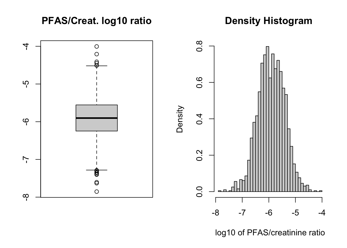

Figure 7.1: Boxplot and histogram of log10 transformation of PFAS sum data after creatinine adjustment.

par(mfrow=c(1,1))

7.5 Exposure - Outcome

Background²⁴: “The key to understanding the environmental fate and transport of PFAS compounds is their surface-active behavior. The fluorinated backbone is both hydrophobic (water repelling) and oleophobic/lipophobic (oil/fat repelling) while the terminal functional group is hydrophilic (water loving). This means that PFAS compounds tend to partition to interfaces, such as between air and water with the fluorinated backbone residing in air and the terminal functional group residing in water. The PFAS partitioning behavior also is affected by the alkyl chain length and the charge on the terminal functional group. In general, PFASs with shorter alkyl chain length are more water soluble than those with longer lengths.”

One question that may arise is whether PFAS compounds could accumulate in the fat tissue in the body. We can explore this option thanks to the “Body Measures (BMX_I)” NHANES data, at least on a broad sense. But we first need to download the file:

#BMX_I - 1.9 MB
download.file("https://wwwn.cdc.gov/nchs/nhanes/2015-2016/BMX_I.XPT", 
              tf <- tempfile(), 
              mode="wb")
BMX_I <- foreign::read.xport(tf)
# Dimensions
dim(BMX_I)

[1] 9544   26

For this test we’ll only keep the BMXBMI column “*Body Mass Index (kg/m**2)*” which is the 11^th column. We also need to keep the common SEQN column. We can merge these 2 columns with the dataset containing the creatinine adjustment of the PFAS sum data we just made earlier:

PFAS_CRE_BMI <- merge(PFAS_CRE, BMX_I[, c(1,11)], by.x = "SEQN", by.y = "SEQN")

We can take a quick look at the BMI distribution with original and log10 values in a histogram form:

par(mfrow=c(1,2))
with(PFAS_CRE_BMI,hist(BMXBMI, breaks = 30))
with(PFAS_CRE_BMI,hist(log10(BMXBMI), breaks = 30)) ; par(mfrow=c(1,1))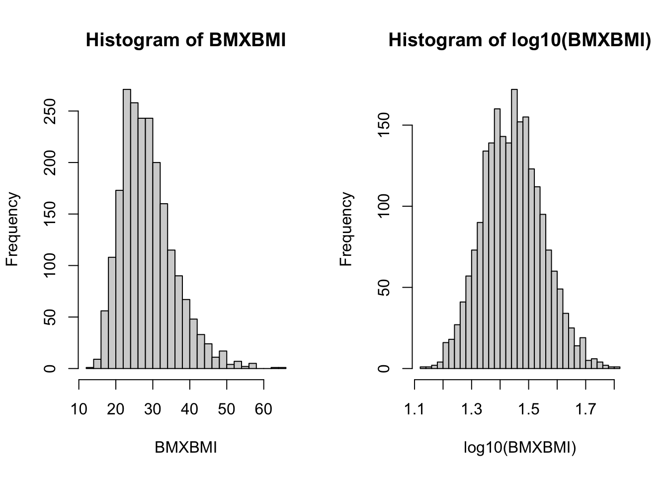

Figure 7.2: Histogram of BMI values and log10 values.

We can note that, as would be expected,the logged values have a more “bell-shaped”distribution.

We can now create a simple plot showing PFAS values as a function of BMI. We can plot both the original values as well as the log values.

par(mfrow=c(1,2))
with(PFAS_CRE_BMI, plot(BMXBMI ~ LBXMFOS))
with(PFAS_CRE_BMI, plot(log10(BMXBMI) ~ log10(LBXMFOS))); par(mfrow=c(1,1))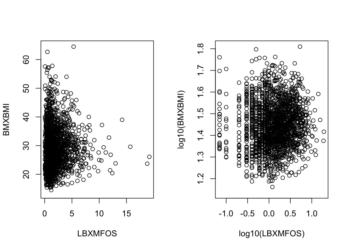

Figure 7.3: Histogram of BMI values and log10 values.

We can add a simple linear regression line for both plot as we have seen previously (section 5.7.)

lm1 <- with(PFAS_CRE_BMI, lm(BMXBMI ~ LBXMFOS))
lm2 <- with(PFAS_CRE_BMI, lm(log10(BMXBMI) ~ log10(LBXMFOS)))
# print out values
lm1; lm2


Call:
lm(formula = BMXBMI ~ LBXMFOS)

Coefficients:
(Intercept)      LBXMFOS  
    28.5857       0.1376


Call:
lm(formula = log10(BMXBMI) ~ log10(LBXMFOS))

Coefficients:
   (Intercept)  log10(LBXMFOS)  
        1.4458          0.0154

abline(lm1, col="blue", lwd=3)
abline(lm2, col="blue", lwd=3)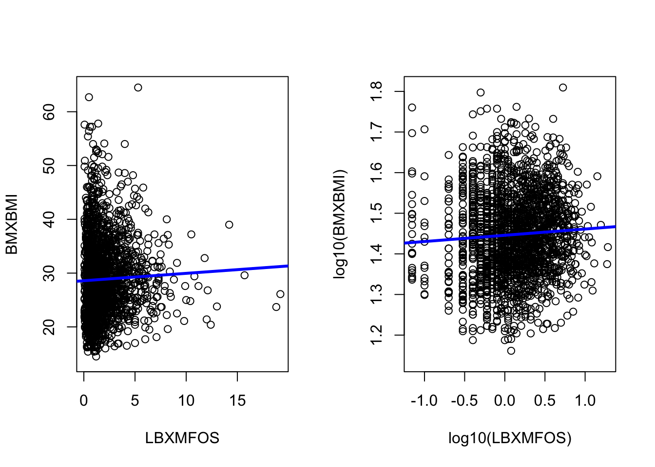

Figure 7.4: Histogram of BMI values and log10 values with added linear regression.

The slope in faint in both cases and indeed the slope values found in the coefficients records (section 5.7) are low at about 0.138 for the normal values and 0.015 for the log values.

We can confirm that the correlation is faint by calculating the Pearson correlation factor which is the default method for the cor() function. The help tells us that we need to add use="complete.obs" to the command to avoid an NA result or errors due to missing values.

with(PFAS_CRE_BMI, cor(BMXBMI ,LBXMFOS, use="complete.obs"))

[1] 0.03611288

with(PFAS_CRE_BMI, cor(log10(BMXBMI) ,log10(LBXMFOS), use="complete.obs"))

[1] 0.05981631

The values are indeed very small in accord with the very flat linear regression.

7.5.1 Illusions

It can be noted that if the plot is stretched horizontally, the line will look even flatter. The can be seen if we change the plotting position with par(mfrow=c(2,1)) instead of par(mfrow=c(1,2)).

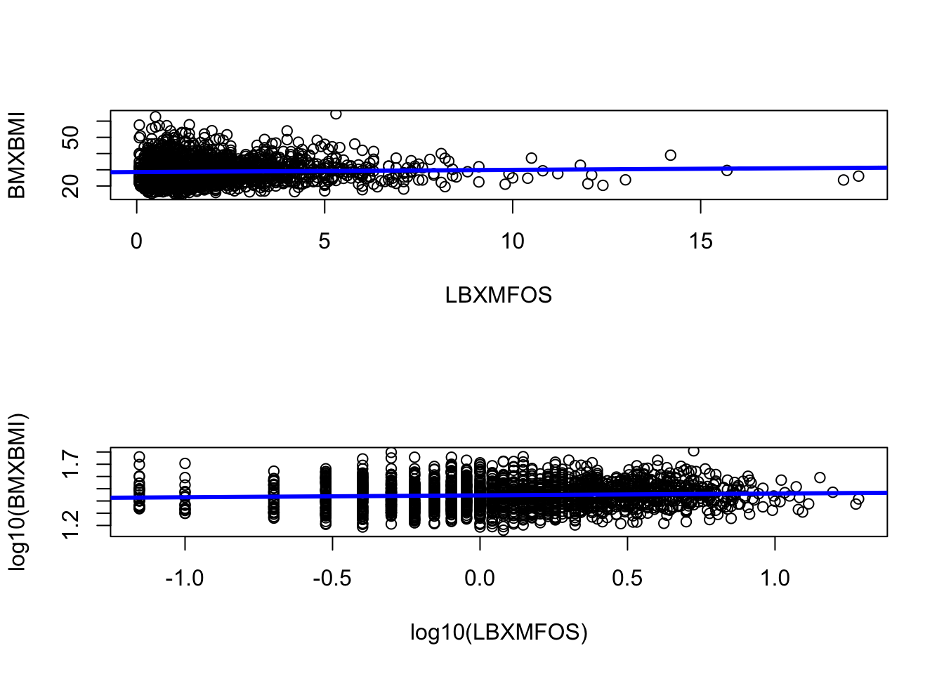
Figure 7.5: Streching horizontally makes the linear regression appear more horizontal

7.5.2 qplot version

The qplot() version can be created by getting inspired to what was done in section 5.8.2.

`geom_smooth()` using formula 'y ~ x'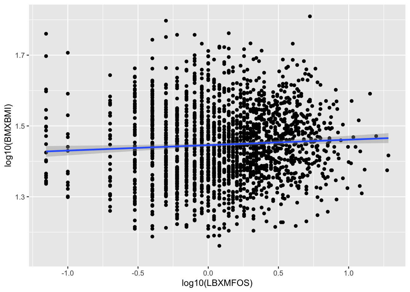

Figure 7.6: Histogram of BMI log10 values, linear regression (blue) and standard error (gray.)

7.6 Creating a master data file

See Appendix D for a complete set of code to download, merge and save the master file.

We have learned how to combine two NHANES data files, but it is could useful to be able to merge more data into a large repository or “master” file from which smaller datasets can be created.

The merge() function can automatically recognize identical columns which will make the merging easier as it will not be necessary to use the by.x commands. In fact, doing so will prevent the merge() function to recognize columns that are identical and this will result in duplicate columns. However, to make the file a “master* we would need to keep all rows, and this is accomplished by adding the all.x option (see ?merge.) Below we’ll download and merge more datasets, including some that we already have downloaded. This should just be a review.

We’ll add the file BMX_I for body/mass index and other body measurements as well as the demographic file DEMO_I and the PFAS_I,

# DEMO_I - 3.6 MB
download.file("https://wwwn.cdc.gov/nchs/nhanes/2015-2016/DEMO_I.XPT", 
              tf <- tempfile(), 
              mode="wb")
DEMO_I <- foreign::read.xport(tf)
# Dimensions
dim(DEMO_I)

[1] 9971   47

We previously downloaded (or learned how to download) the albumin/creatinine file (ALB_CR_I) and that of total cholesterol TCHOL_I.

Let’s merge all 4 keeping all rows starting with DEMO_I so that it is on the left hand side.

Master1 <- merge(DEMO_I, BMX_I, all.x=TRUE)
Master2 <- merge(Master1, PFAS_I, all.x=TRUE)
Master3 <- merge(Master2, TCHOL_I, all.x=TRUE)
Master4 <- merge(Master3, ALB_CR_I, all.x=TRUE)
# dimensions
dim(Master1) ; dim(Master2);  dim(Master3);  dim(Master4)

[1] 9971   72

[1] 9971   93

[1] 9971   95

[1] 9971  102

The process would be the same to add more data file.

To save the master file into a comma separated file (.csv) use the write_csv() function of dyplr which is “about twice as fast as write.csv(), and never writes row names.” (See chapter 8 section 8.3 and chapter (10 as we have not yet studied that package at this point.)

For example to save the data frame Master4 in the current directory:

write_csv(Master4, "Master4.csv")

Using base R we would write similarly:

write.csv(Master4, "Master4.csv")

This would allow to read the data again without having to go through the process of creating the combined dataset.