
Chapter 6 Importing data
Importing data is rather easy in R but that may also depend on the nature of the data to be imported and from what format. For environmental studies data are usually in tabular form such as a spreadsheet or a comma-separated file (.csv.)
In this chapter:
- Importing from local files
- Downloading Nhanes data
- Exploring PFAS_I data
- Merging data files
The way or method used to import the data in R will have fundamental implications on the class of the object containing the data just read and therefore what methods can later be used to analyze the data. In Classic R we’ll most likely want to have the data in the data.frame class as it is the most versatile and useful.
Base R has a series of read functions to import tabular data from plain text files with columns delimited by: space, tab, comma, with or without a header containing the column names. With an added package it is also possible to import directly from a Microsoft Excel spreadsheet format or other foreign formats from various sources.
6.1 Importing from local files
In base R the standard commands to read text files are based on the read.table() function. The derived functions exist in 2 flavor to accommodate USA and European conventions for decimal point (a comma in Europe) and comma separator (a semicolon in Europe.) The following table lists the collection of the base R “read” functions. For more details use the help command help(read.table) that will display help for all.
| Function name | Assumes header | Separator | Decimal | File type | Comment |
|---|---|---|---|---|---|
read.table() |
No | none | . |
.txt |
USA |
read.csv() |
Yes | , |
. |
.csv |
USA |
read.csv2() |
Yes | ; |
, |
.csv |
Europe |
read.delim() |
Yes | Tab | . |
.txt |
USA |
read.delim2() |
Yes | Tab | , |
.txt |
Europe |
A similar approach is used to write the data out but the *delim() version do not exist, but can be managed with specifying the tab delimiter within the write.table() function.
Assuming that you have a file name test.csv containing these 5 columns of data
c1,c2,c3,c4,c5
1.481,3.478,4.246,3.687,6.051
1.73,5.825,4.526,6.754,0.15
2.556,6.275,2.525,6.368,5.479
2.828,4.77,5.12,3.744,4.01
2.989,4.396,2.078,4.237,4.618
3.122,6.317,5.414,3.551,5.607
The command to read such a file into a user defined object named test would be:
# Do not run
test <- read.csv("test.csv")
6.2 Downloading Nhanes data
R is a great “statistical software for data analysis” but there are other competing software in Industry that can even be expensive such as SPSS, STATA, JMP, Matlab, and SAS.
NHANES data is saved in a SAS transport file (.xpt) created by the SAS XPORT engine. This is what is available on the NHANES web site. Fortunately they also provide methods to import this data in R by using the foreign package (see Appendix C.)
TASK: Install package. foreign.
It is necessary to install this package to be able to follow the code below and import the NHANES data. You can use install.packages("foreign") or follow alternate direction in section 1.2.
See also Appendix D.4 for an alternate method using the haven package instead. See Appendix D.5 for code to download and save .XPT files onto your computer.
Relax
You may be given a pre-downloaded data set for your homework exercise(s).
However, it is always useful to know where and how to get your own data. This is the purpose of this section.
Other options See Appendix D and section 6.4 for more details.
The relevant .XPT files used in this book were combined into a .zip archive that can be downloaded: XPTs.zip
The combined “Master4” file can also be downloaded as well as a .csv file with either:
6.2.1 PFAS_I

Figure 6.1: Perfluorooctanoic acid (PFOA) is used worldwide as an industrial surfactant in chemical processes and as a material feedstock, and is a health concern and subject to regulatory action and voluntary industrial phase-outs.
As an example we’ll download the file resulting of the blood serum analysis of Perfluoroalkyl and Polyfluoroalkyl substances (PFAS_I) used in multiple commercial applications including surfactants, lubricants, paints, polishes, food packaging and fire-retarding foams. More information can be read from the documentation page15 (that also contains a link describing all the details for the laboratory methods used.)
For more information:
Perfluoroalkyl and Polyfluoroalkyl Substances16 on NIEHS / NIH web site.
Perfluoroalkyl and Polyfluoroalkyl Substances in the Environment: Terminology, Classification, and Origins17 by Buck et al. (2011). (See their Table 1 in Appendix F.)
The NHANES tutorial R code (Appendix C) is for the demographic data in file DEMO_I.XPT:
# DO NOT RUN
# Download NHANES 2015-2016 to temporary file
download.file("https://wwwn.cdc.gov/nchs/nhanes/2015-2016/DEMO_I.XPT",
              tf <- tempfile(),
              mode="wb")

# Create Data Frame From Temporary File
DEMO_I <- foreign::read.xport(tf)
The first command using the download.file() function accomplishes 2 tasks, it will:
- download the file from the web link
- save the file to a temporary file named
tf, using the transfer mode codedwfor write andbfor binary. (For more info see detail on file openfopenoptions 18.)
This “trick” avoids saving the file locally to the hard drive. Should one want to do that the command could be simplified by replacing tf <- tempfile() with the name of a file within quotes such as DEMO_I.XPT.
The second command uses the foreign package function read.xport() to read the data into a data frame named DEMO_I. If we had saved the file to the local drive we would replace tf with DEMO_I.XPT.
NOTATION: The use of :: notation in foreign::read.xport(tf) tells R to use the function read.xport() from the foreign package without the need to use the library() function first. This is common for cases where we only want to use a function once.
Alternate package: An alternate option to the code provided is using the package haven and download the file instead with:
DEMO_I <- read_xpt(url(
"https://wwwn.cdc.gov/Nchs/Nhanes/2015-2016/DEMO_I.XPT"))
The data can be found on the web site starting at: https://wwwn.cdc.gov/nchs/nhanes/ContinuousNhanes/ and then:
- Click on “Laboratory data” (figure 6.2)
- Scroll and find the 2015-1016 entry
The entry is specified to be only 376.7 Kb in size.
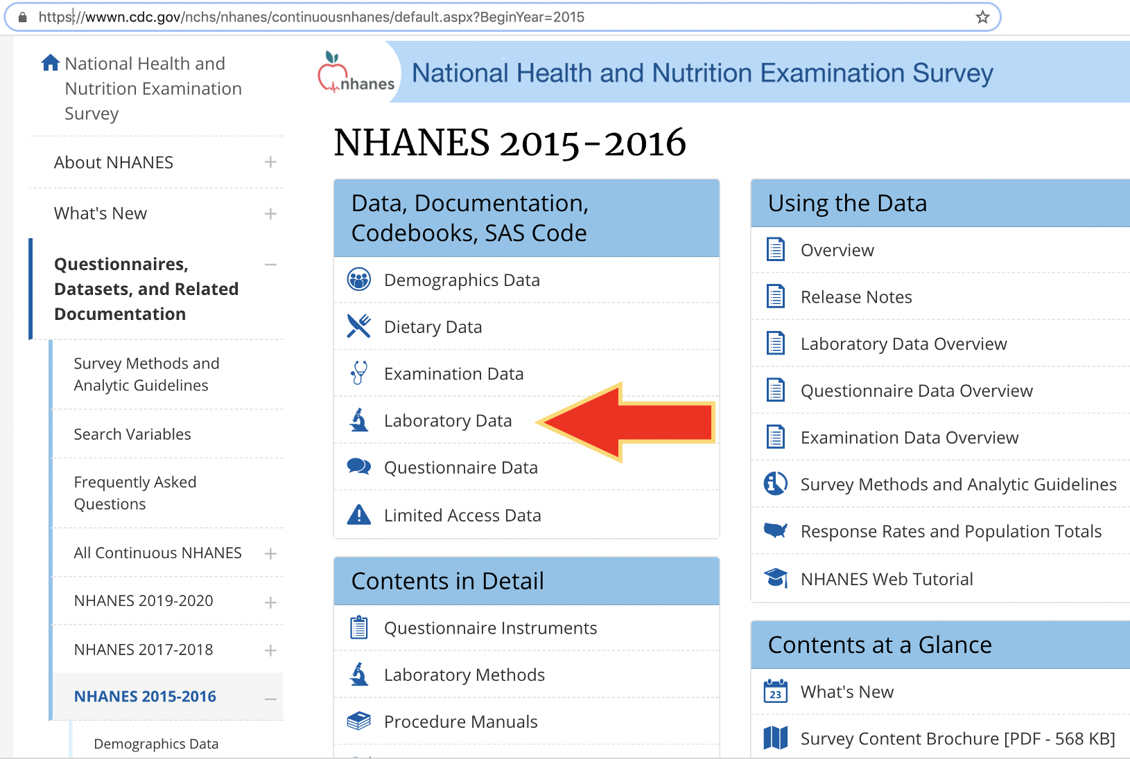
Figure 6.2: Finding NHANES 2015-2016 data.
TASK: Download file PFAS_I.XPT.
The data file direct link is:
https://wwwn.cdc.gov/nchs/nhanes/2015-2016/PFAS_I.XPT
We can download the file as in the above example without the need to save the .XPT file on the local drive.
# Download NHANES PFAS_I 2015-2016 data to temporary file
download.file("https://wwwn.cdc.gov/nchs/nhanes/2015-2016/PFAS_I.XPT",
              tf <- tempfile(),
              mode="wb")

# Create Data Frame PFAS_I From Temporary File
PFAS_I <- foreign::read.xport(tf)

class(PFAS_I)
[1] "data.frame"We now have a data frame named PFAS_I.
6.3 Exploring PFAS_I data
PFAS_I is of class data.frame. The meaning of the column headers can be found in the NHANES documentation page https://wwwn.cdc.gov/Nchs/Nhanes/2015-2016/PFAS_I.htm (also found in Appendix E.)
The first and last three codes are in the table shown here.
| Code | Description |
|---|---|
| SEQN | Respondent sequence number |
| LBXMFOS | Sm-PFOS (ng/mL) |
| LBDMFOSL | Sm-PFOS Comment Code |
If we read the code information on the web page or on Appendix E we can see that some columns are “comment” columns. These report the “success” of the analysis with a value of 0 at or above the detection limit, a value of 1 below lower detection limit and a dot . for missing values. One more thing to notice is that the text entry describing these columns is written in multiple ways:
- Comment Code: 5 times
- Comt Code: 4 times
- comment : 1 time
Therefore there are 10 “comment” columns that alternate with data columns.
We can also note that the data columns all contain an X in their name while the comment columns contain the letter D. The first 2 columns of SEQN and WTSB2YR are not part of that naming pattern.
REVIEW classic R methods:
This is the perfect time to review the classic methods that are built-in R that we explored with the airquality dataset with functions:
dim(), length(), str(), summary(), colnames(), head() and tail(), colSums(is.na()). etc.
Since they were already visited those exact commands will not be developed again but we’ll see how to do some specific manipulations by adding optional arguments in some of the commands.
We’ll start by exploring the data graphically.
6.3.1 PFAS_I boxplot
The base R graphics functions are rather smart to make a graph quickly with little information. We could for example use boxplot(PFAS_I) but we would quickly note that the first column SEQN would “crush all other columns simply because the values for this column that represents the”Respondent sequence number” (the code for each individual) has range 83736 to 93700 as reported by command summary(PFAS_I[,1]). Therefore as a first approach it would be useful to be able to plot everything without the first column. This is accomplish with subsetting (section 5.3) but using a minus sign to indicate that we want to remove the designated column. The command to remove the first command would be:
# Remove the first columns
boxplot(PFAS_I[, -1])
We just need to remember that within the square brackets the first item represents rows and the second represents columns. Nothing written means take everything. In that sense PFAS_I[ , ] is exactly the same as simply PFAS_I. We just specify -1 for columns to remove the first one.
However, the next “annoying” thing will be that data from column 2 is now “crushing” the other boxes So we now want to remove the first 2 columns: SEQN and WTSB2YR. How do we do that? there are only 2 spots within the square bracket.
To remove the 2 columns we can take advantage of the combine function c() to gather the numbers of the columns and add a minus sign before it to specify their removal. We can thus write:
# Remove the first and second columns
boxplot(PFAS_I[, -c(1:2)])
This is still not satisfying as there are a lot of “outliers” i.e. values that extend beyond the box. And once again the boxes are all “crushed”.
One way to have a better image is to limit the values that are plotted in the vertical (y) axis by using the optional parameter ylim = which requires 2 numbers specifying a lower and an upper limit, for example from 0 to 10. Note that once again we need to use the combine c() function, something that is ubiquitous in R code:
# Remove the first and second columns
# limit vertical axis with ylim
boxplot(PFAS_I[, -c(1:2)], ylim = c(0,10))
All four attempts can be summarized as:
par(mfrow =  c(2,2))
# All data
boxplot(PFAS_I)
# Remove the first columns
boxplot(PFAS_I[, -1])
# Remove the first and second columns
boxplot(PFAS_I[, -c(1:2)])
# limit vertical axis with ylim
boxplot(PFAS_I[, -c(1:2)], ylim = c(0,10))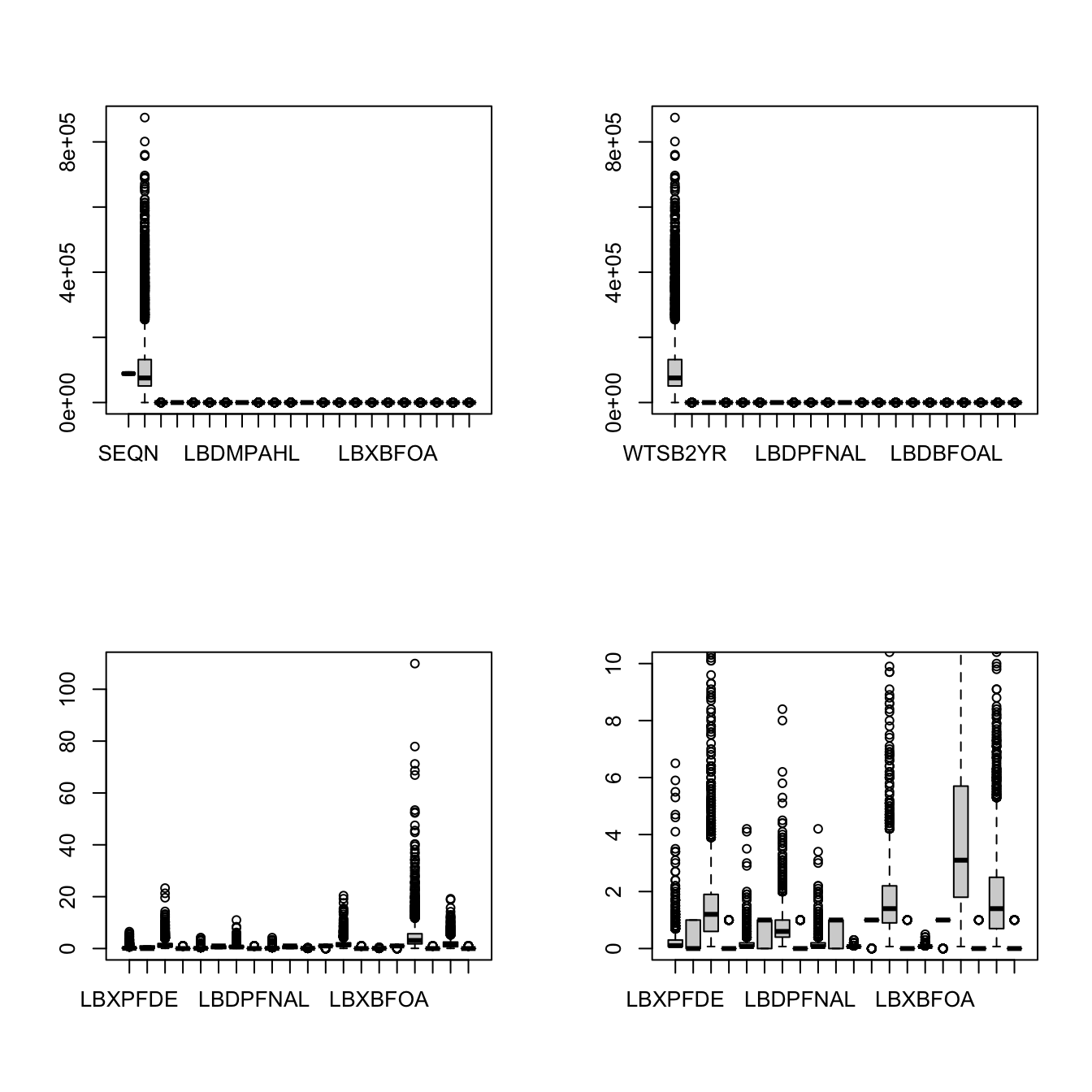
Figure 6.3: Summary of 4 attempts
par(mfrow = c(1,1))This has not been so useful yet, but we are getting closer perhaps!
We noted earlier (section 6.3) that besides the first 2 columns, every other column was a “comment” column containing only 0, 1, anda few .. Therefore it is not very useful to include them in the plot. We can further realize that they are all columns with an odd number, and we can create a list of these numbers from the seq() function (section 4.8.1).
We want to omit columns 1 and 2, and finish with column 21 since the last column 22 is a “comment” column. So starting with 3 and stepping by 2 will provide all odd numbers between 3 and 21.
seq(3,21, by = 2) [1] 3 5 7 9 11 13 15 17 19 21We can also remember that using a log() function may give the data a better spread. If this does not work for the boxplot perhaps it will work for a histogram. We could also noted in the previous attempts that the labels for the columns are printed on the horizontal axis, but not all of them due to spacing. We can therefore add an additional option which will rotated the bottom labels by 90 degrees so that all of them can be printed. To find this option one would have to learn about it in an example, as finding it by help is tricky unless we know where to look, which would be the list of paramters for graphics found with help(par). The command is las=2 and that is most likely an abbreviation for label axis style.
The following command combines all of that. We are asking for a boxplot from PFAS_I, the values will be changed to the natural log, only for columns that are odd and the label will be rotated on the horizontal axis:
boxplot(log(PFAS_I[, seq(3,21, by = 2)]), las=2)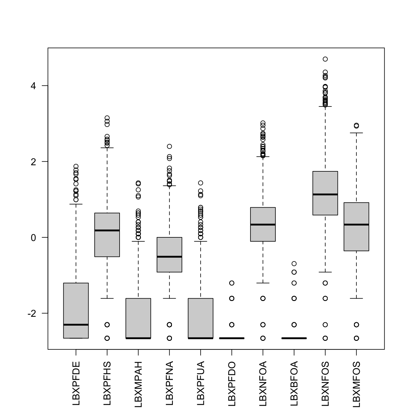
Figure 6.4: PFAS_I boxplot with log values for odd columns and rotated labels.
There are many fancy ways to alter base R graphics, a very detailed example can be found in this blog19 or this published “excercise” Fixing Axes and Labels in R Plot Using Basic Options20.
However, most people now are switching to more modern plotting methods for making the final, fancy or published version. However, it is still very useful to know how to use R base graphics to explore data as they are usually simpler to apply at first.
6.3.2 PFAS_I histogram
We can perhaps quickly apply what we just learned to making histograms of the data.
The difference here is that each histogram would need to be a separate graph. So just replacing boxplot by hist will not work.
Let’s start by looking at just one of them. Column 21 is the sum of all others. We can test also if it is necessary to use the log() function. We can plot both original and logged values in one image. We can also use remember and use the other subset method using the with() function which will make the title of the plot nicer (see (section 5.4.)
par(mfrow =  c(1,2))
# original data
# hist(PFAS_I[,21])
with(PFAS_I, hist(LBXMFOS))
# natural log applied
# hist(log(PFAS_I[,21]))
with(PFAS_I, hist(log(LBXMFOS)))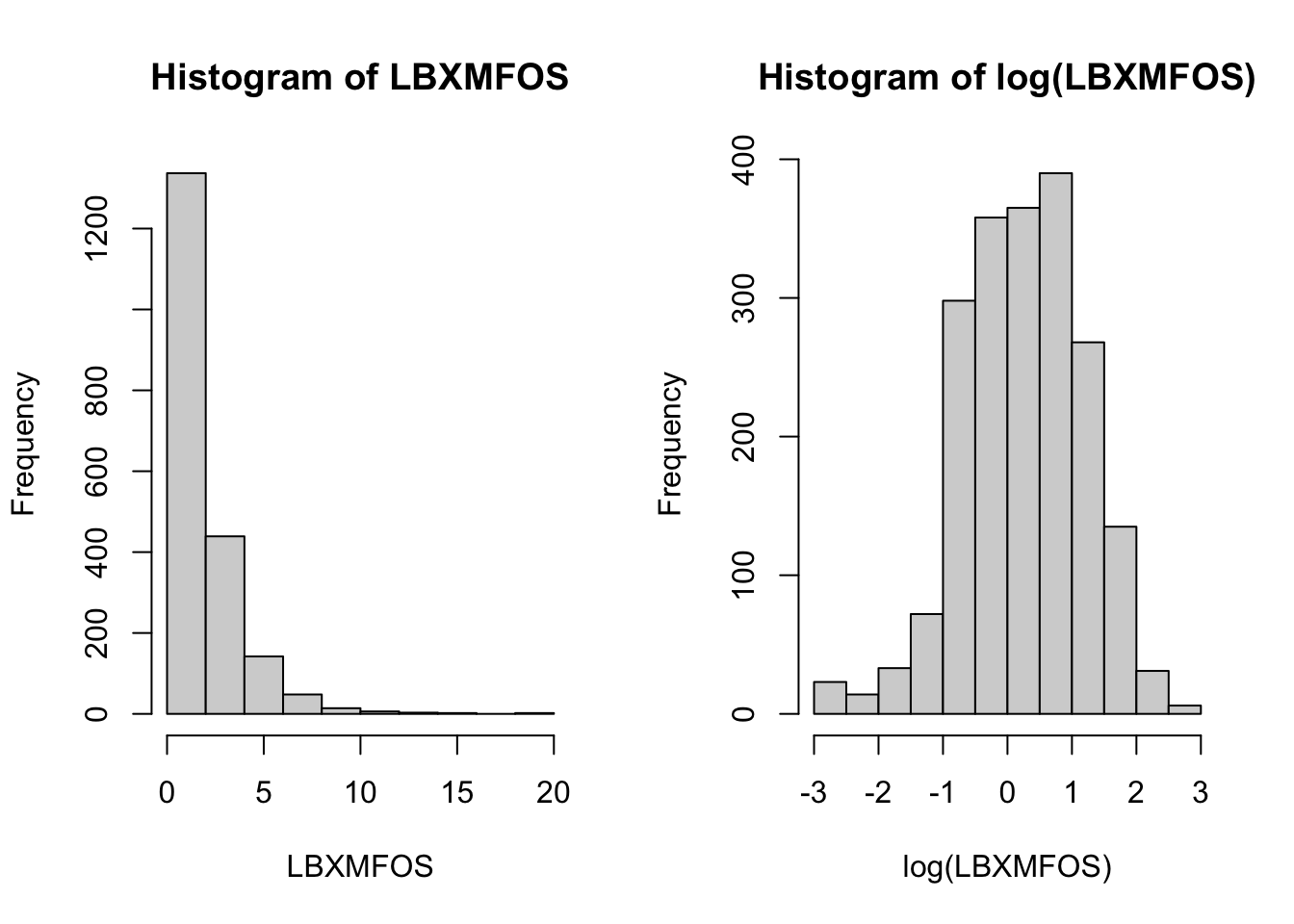
Figure 6.5: PFAS_I histogram for summed values in column 21 labeled LBXMFOS.
par(mfrow = c(1,1))NOTE
For histograms the options breaks = 25 could be added (possibly with a different number) to bin into smaller portions and make a finer plot.
By default the histogram will be a “frequencies” version that can be changed to a “densities” version so that the histogram has a total area of one. This is done by adding freq = FALSE. See help(hist).
So how do we plot all of the histograms for all columns? This is more complicated that it appears at first thought. On discussion forums it would be possible to find answers that have R code on many lines looking like a full program. However, there is a simple solution but it uses a rather challenging base R function that is difficult to understand for most people.
It would be very difficult to also apply the log() function to the data. Let’s create a small subset of 4 of the 10 data columns. We’ll store that data in a simple named object L after which we can verify some properties:
L <- log(PFAS_I[, c(5,9,15,21)])
class(L)
[1] "data.frame"colnames(PFAS_I[, c(5,9,15,21)])[1] "LBXPFHS" "LBXPFNA" "LBXNFOA" "LBXMFOS"Taking into account that we’ll have 4 plots the “magical” command is now simply: lapply(L, hist).
par(mfrow =  c(2,2))
lapply(L, hist)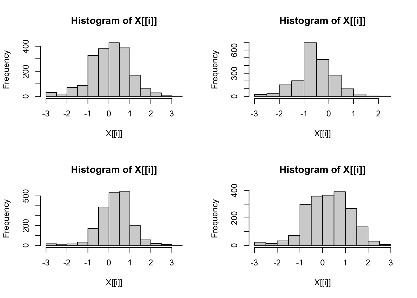
Figure 6.6: Creating multiple histograms with one command
par(mfrow = c(1,1))Some additional options can be added to change the historgram but the format is different that when the hist() function is used. In this case the additional parameters would need to follow hist separated by a comma. For example to add 2 parameters:
lapply(L, hist, breaks=25, freq = FALSE).
Each title “Histogram of X[[i]]” could be changed to the same title for all with e.g. main = "Histogram" or compltely suppressed with main = "". But to provide the name of the column either in the title or on the axis would require even more sophisticated commands.
ADVANCED
The solution for this calls on the lapply() function that can be difficult to understand. This whole family of functions is described in details on the guru99 web site:
https://www.guru99.com/r-apply-sapply-tapply.html
These functions can be very useful and are found as suggestions on forums.
6.3.3 Fancier boxplot with qplot
This section uses ggplot2 which is a package included in the Tidyverse suite. If you need to install this go to section 1.2 and proceed with the installation.
This section is here to illustrate another way to create the same or similar plots as we did with base R. It may be confusing at first, in which case this section can be skipped to better come back later. Perhaps after learning more from links in chapter 11.
Most ggplot examples online assume that some of the columns of the data can be used to plot against other columns as we did for the airquality plots using the easier qplot() (section 5.8.)
The data we have in PFAS_I are all number data and we’d like to plot them all as we did with the base R graphic function boxplot().
This section with a quick solution is here as it is difficult to find examples that match the data style we have here i.e. many columns that need to be plotted. The solution involves the stack() function that is part of the utils “utilities library” for data frames.
This solution was found on this forum page: Building a box plot from all columns of data frame with column names on x in ggplot221.
To understand what it does we can simply look at its effect on the L object:
head(stack(L)) values ind
1 -0.5108256 LBXPFHS
2 0.3364722 LBXPFHS
3 1.5892352 LBXPFHS
4 0.1823216 LBXPFHS
5 -1.6094379 LBXPFHS
6 -0.6931472 LBXPFHSNote: this could be written head(utils::stack(L)) in case of ambiguity with other commands.
The effect is to create a simpler but longer format as long as the number of columns multiplied by the number of rows. For L this would be 2170 * 4 = 8680. The column names for this format is always values and ind (independent variable) which are names to be reported in qplot():
# library(ggplot2)
qplot(ind, values, data = stack(L), geom = "boxplot")
Warning: Removed 708 rows containing non-finite values (stat_boxplot).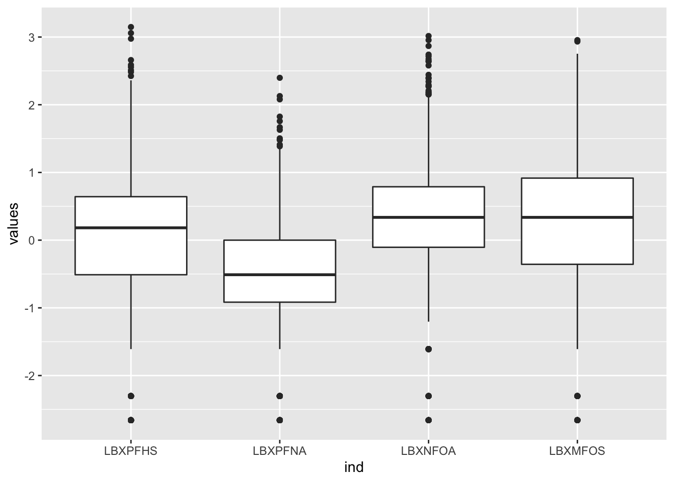
Figure 6.7: PFAS_I boxplot with log values for 4 columns.
We’ll see later how this work, but the ggplot version for all 10 odd-numbered columns could be written as:
# library(ggplot2)
ggplot(stack(log(PFAS_I[, seq(3,21, by = 2)])),
       aes(x = ind, y = values)) +
  geom_boxplot()
Warning: Removed 1770 rows containing non-finite values (stat_boxplot).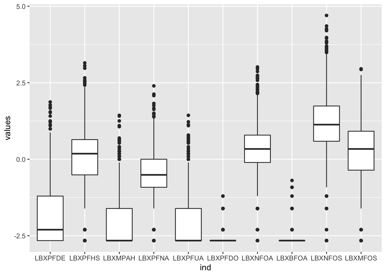
Figure 6.8: PFAS_I boxplot with log values for 10 data columns.
6.4 Merging data files

Figure 6.9: Combining NHANES data into a single file is necessary for detailed analysis.
NHANES data are split into multiple files to provide flexibility and modularity in the choice of data. This makes the data easier to handle in small portions rather than a huge, single data file. On the other hand it is often necessary to merge one or more data file in order to obtain all of the data required for an analysis so that all of the data for an individual scattered among multiple files be found on a single row in the new, combined data file.
All that is required and necessary to merge data is at least a single column with the same name. All NHANES data pertinent to individuals (excluding special files with pooled data) start with the SEQN column that identify individuals with a unique number.
PFAS may disrupt lipid regulation and gathering data that have both PFAS and cholesterol or triglyceride data would help in a study. As an example we’ll merge the PFAS_I file with another file containing cholesterol data. There are 3 files containing cholesterol data for 2015-2016, separated by type.
| Data File Name | Doc File | Data File | Date Published |
|---|---|---|---|
| Cholesterol - High-Density Lipoprotein (HDL) | HDL_I Doc | HDL_I Data [XPT - 189.2 KB] | September 2017 |
| Cholesterol - Low - Density Lipoprotein (LDL) & Triglycerides | TRIGLY_I Doc | TRIGLY_I Data [XPT - 151.2 KB] | January 2019 |
| Cholesterol - Total | TCHOL_I Doc | TCHOL_I Data [XPT - 189.2 KB] | September 2017 |
The number of observation within each file is different with 8021 (765 missing) for both total cholesterol and HDL files, and only 3191 (468 missing) for LDL + Triglyceride. The latter is probably due to NHANES method to use subsets of a population as a cost saving method.
The PFAS_I data contains 2170 entries with 177 missing. During the merging of the data, only rows that have a corresponding SEQN entry will be saved.
For simplicity we’ll use the total cholesterol data. It contains only three columns but none of them are “comment” columns:
SEQN- Respondent sequence numberLBXTC- Total Cholesterol (mg/dL)LBDTCSI- Total Cholesterol (mmol/L)
The LBDTCSI variable was derived from LBXTC: The total cholesterol in mg/dL (LBXTC) was converted to mmol/L (LBDTCSI) by multiplying by 0.02586.
The file has to be downloaded into a new user-defined R object as we did with the PFAS data:
# Download NHANES TCHOL_I 2015-2016 data to temporary file
download.file("https://wwwn.cdc.gov/nchs/nhanes/2015-2016/TCHOL_I.XPT",
              tf <- tempfile(),
              mode="wb")

# Create Data Frame PFAS_I From Temporary File
TCHOL_I <- foreign::read.xport(tf)

class(TCHOL_I)
[1] "data.frame"6.4.1 Merge() function
The merge() function has many optional parameters that permit variations of the merging. Details on all options for this function are available as help(merge) or simply ?merge.
All we want for now is specify a common column, in our case SEQN and just keep the entries that exist for both data files. Therefore the total number of entries cannot be larger than that of PFAS_I, that is 2170.
The specification of the chosen columns is done with the by.x and by.y options. In our case the chosen name will be the same. But if by chance the name was different in the 2 files, specifying the name of the column in this way would still work.
So, let’s combine the 2 files:
# Merging PFAS and total cholesterol TCHOL data frames
M1 <- merge(PFAS_I, TCHOL_I, by.x = "SEQN", by.y = "SEQN")

class(M1)
[1] "data.frame"dim(M1)[1] 2170 24Since TCHOL_I is the second argument (y in documention) its columns are added at the end of PFAS_I. Inverting the arguments would place the TCHOL_I columns at the beginning. However, in all cases the SEQN column remains the first column.
We can check the name of just a few columns, for example with:
colnames(M1)[c(1,20:24)][1] "SEQN" "LBDNFOSL" "LBXMFOS" "LBDMFOSL" "LBXTC" "LBDTCSI" The last 2 names are indeed the code names found in the documentation for TCHOL_I.
We now have merged 2 data files using the unique number for each individual. The process would be the same to add more data, for example adding the other cholesterol data files for HDL and LDL+Triglycerides. But this can be done as an exercise if it proves useful.

Figure 6.10: We have combined NHANES data for each individual from 2 separate files.
6.4.2 Merging demographics data
Most studies are set to compare and analyze data for different population. Therefore adding the “demographics” data file would be useful.
Study: Merge your data with the demographics file if your study requires it.
The procedure would be exactly the same using the merge() function through the common SEQN column for individuals.
The code to download the demographics data was the example we saw earlier in section 6.2.1.
